Fangzhou Cheng

Introduction:

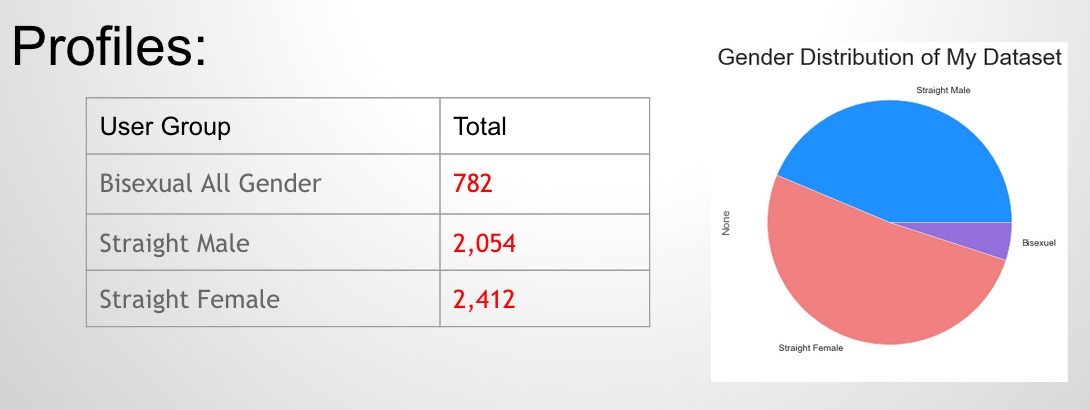
40 million Americans indicated that they used online dating services at least once in their life (source), which got my attention — Who are these people? How do they behave online? Demographics analysis (age and location distribution), along with some psychological analysis (who are pickier? who are lying?) are included in this project. Analysis is based on 2,054 straight male, 2,412 straight female, and 782 bisexual mixed gender profiles scraped from Okcupid.

Project Introduction: project information and data analysis deck
Project Source Code: project source code
Github Repo: https://github.com/funjo/okcupid_scraper

We found love in a hopeless place

• 44% of adult Americans are single, which means 100 million people out there!
  • in New York state, it’s 50%
  • in DC, it’s 70%
• 40 million Americans use online dating services.That’s about 40% of our entire U.S. single-people pool.
• OkCupid has around 30M total users and gets over 1M unique users logging in per day. its demographics reflect the general Internet-using public.

Step 1. Web Scraping

1. Get usernames from matches browsing.

• Create a profile with only the basic and generic information.
• Get cookies from login network response.
• Set search criteria in browser and copy the URL.

First, get login cookies. The cookies contain my login credentials so that python will conduct searching and scraping using my OkCupid username.

from bs4 import BeautifulSoup
import requests
import re
import pandas as pd
import csv
import matplotlib.pyplot as plt
import seaborn as sns
from geopy.geocoders import Nominatim
import string
import numpy as np
import scipy as sp
from scipy import stats
%pylab inline

# get login cookies
def getCookies():
   req = requests.post('https://www.okcupid.com/login',\
   data={'login_username': 'uhohcantletyouknow', 'login_password':'uhohcantletyouknow'})
   cookies = req.cookies
   return cookies
cookies = cookies

Then define a python function to scrape a maximum of 30 usernames from one single page search (30 is the maximum number that one result page can give me).

# get a maximum of 30 usernames from one search
def getUsernames():
   url = 'http://www.okcupid.com/match?filter1=0,48&filter2=2,100,18&filter3=5,2678400&filter4=1,1&locid=0&timekey=1&matchOrderBy=SPECIAL_BLEND&custom_search=0&fromWhoOnline=0&mygender=m&update_prefs=1&sort_type=0&sa=1&using_saved_search=&count=30'
   page = requests.get(url, cookies = cookies).text
   soup = BeautifulSoup(page, 'html5lib')
   result = soup.find_all('div', {'class':'match_card_wrapper user-not-hidden '})
   roughnames = [i.get('id') for i in result]
   usernames = [re.findall('usr-(.*)-wrapper', i)[0] for i in roughnames]
   return usernames

Define another function to repeat this one page scraping for n times. For example, if you set 1000 here, you’ll get roughly 1000 * 30 = 30,000 usernames. The function also helps picking out redundancies in the list (filter out the repeated usernames).

# repeat the above search multiple times
def getLotsUsernames():
   usernames = []
   for i in range(1000):
   # 1000 pages * 30 usernames per page = about 30,000 usernames
       usernames += getUsernames()
       print 'Scraped', i, 'of 1000 targeted pages.'
   unique = set(usernames)
   print 'Downloaded %d usernames, of which %d are unique.' % (len(usernames), len(unique))
   return unique

%%time
usernames = getLotsUsernames() usernames = list(usernames)
for i in range(len(usernames)):
   usernames[i] = usernames[i].encode('utf-8')

Export all these unique usernames into a new text file. Here I also defined a update function to add usernames to an existing file. This function comes in handy when there are interruptions in the scraping process. And of course, this function handles redundancies automatically for me as well.

# write usernames into new file
def writeUsernames(usernames):
   string = ''
   for i in usernames:
       string += i+'\n'
   with open('usernames.txt', 'w') as f:
       f.write(string)
   print len(usernames), 'of usernames have been written into usernames.txt.'

# rewrite the file with unique usernames if redundancies are found after multiple scraping attempts
def appendUsernames(usernames):
   string = ''
   for i in usernames:
       string += i+'\n'
   with open('usernames.txt', 'a') as f:
       f.write(string)
   print len(usernames), 'of usernames have been added into usernames.txt.'

appendUsernames(usernames)</pre>

2. Scrape profiles from unique user URL using cookies. www.okcupid.com/profile/username

• User basic information: gender, age, location, orientation, ethnicities, height, bodytype, diet, smoking, drinking, drugs, religion, sign, education, job, income, status, monogamous, children, pets, languages
• User matching information: gender orientation, age range, location, single, purpose
• User self-description: summary, what they are currently doing, what they are good at, noticeable facts, favourite books/movies, things they can’t live without, how to spend time, friday activities, private thing, message preference

Define the core function to deal with profile scraping. Here I used just one python dictionary to store all the information for me (yea, ALL users’ information in one dictionary only). All features mentioned above are the keys in the dictionary. Then I set the values of these keys as lists. For example, person A’s and person B’s locations are just two elements within the long list after the ‘location’ key.

def getProfile(num, username):
   result = {}
   for num in range(num):
       url = 'http://www.okcupid.com/profile/'+username[num]
       test = requests.get(url, cookies = cookies)
       if test.status_code == 200:
           page = requests.get(url, cookies=cookies).text
           soup = BeautifulSoup(page)

           # user basic information
           result.setdefault('username', [])
           result.setdefault('gender', [])
           result.setdefault('age', [])
           result.setdefault('location', [])
           result.setdefault('frequency', [])
           result['username'].append(username[num])
           result['gender'].append(soup.find_all('span',{'class':'ajax_gender'})[0].get_text())
           result['age'].append(soup.find_all('span',{'id':'ajax_age'})[0].get_text())
           result['location'].append(soup.find_all('span',{'id':'ajax_location'})[0].get_text())
           result['frequency'].append(soup.find_all('div',{'class':'tooltip_text hidden'})[0].get_text())

           basic = ['orientation','ethnicities','height','bodytype','diet','smoking','drinking','drugs','religion','sign','education','job','income','status','monogamous','children', 'pets','languages']
           for i in basic:
               result.setdefault(i, [])
               x = soup.find_all('dd', {'id':'ajax_'+i})
           if x == []:
               result[i].append('')
           else:
               result[i].append(x[0].get_text())

           # user matching information
           find = ['gentation','ages','near','single','lookingfor']
           for i in find:
               result.setdefault(i, [])
               x = soup.find_all('li', {'id':'ajax_'+i})
           if x == []:
               result[i].append('')
           else:
               result[i].append(x[0].get_text())

           # user self description information
           text = ['0','1','2','3','4','5','6','7','8','9']
           for i in text:
               result.setdefault(i, [])
               x = soup.find_all('div', {'id':'essay_text_'+i})
           if x == []:
               result[i].append('')
           else:
               result[i].append(x[0].get_text())

         print num, 'of', len(username), test.status_code == 200
     return result

Now, we’ve defined all the functions we need for scraping OkCupid. All we have to do is to set the parameters and call the functions. First, let’s important all the usernames from the text file we saved earlier. Depending on how many usernames you have and how long time you estimate it to take you, you can choose either to scrape all the usernames or just a part of them.

l =[]
with open('usernames.txt', 'r') as f:
   for line in f:
       l.append(line.rstrip('\n'))
s = set(l)
print len(l), 'of usernames have been added to the usernames list.'
print len(s), "of them are unique."

# rewrite the file if there were redundancies
if len(l) != len(s):
   writeUsernames(s)
   print 'usernames.txt file has been rewrriten.'

l = list(s)

# Set the number of usernames to scrape
result = getProfile(len(l), l)

Finally, we can start using some data manipulation techniques. Put these profiles to a pandas data frame. Pandas is a powerful data manipulation package in python, which can convert a dictionary directly to a data frame with columns and rows. After some editing on the column names, I just export it to a csv file. Utf-8 coding is used here to convert some special characters to a readable form.

profile = pd.DataFrame(result)
profile = profile.rename(columns = {'0':'0summary','1':'1doing','2':'2goodat','3':'3notice','4':'4books','5':'5without','6':'6spendtime','7':'7friday','8':'8private','9':'9message'})
profile = profile.set_index(['username'])
print profile.columns

# Export the profiles to csv
profile.to_csv('profile.csv',encoding='utf-8')
!head -5 profile.csv

Step 2. Data Cleaning

• There were a lot of missing values in the profiles that I scraped. This is normal. Some people don’t have enough time to fill everything out, or simply do not want to. I stored those values as empty lists in my big dictionary, and later on converted to NA values in pandas dataframe.
• Encode code in utf-8 coding format to avoid weird characters from default unicode.
• Then to prepare for the Carto DB geographic visualization, I got latitude and longitude information for each user location from python library geopy.
• In the manipulation, I had to use regular expression constantly to get height, age range and state/country information from long strings stored in my dataframe.

Step 3. Data Manipulation

Demographics Analysis

How old are they?

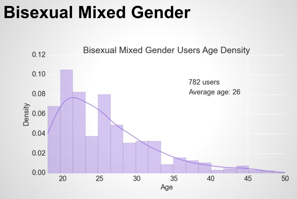
The user age distributions observed are much older than other online reports. This is possibly affected by the login profile setting. I’ve set my robot profile as a 46 year old man located in China. From this we can learn that the system is still using my profile setting as a reference, even if I’ve indicated that I’m open to people from all ages.

# import csv
p = pd.read_table('profiles(male).csv', sep=',')
p.groupby([p.gender]).size()
p2 = pd.read_table('profiles(female).csv', sep=',')
p2.groupby([p2.gender]).size()
p3 = pd.read_table('profile.csv', sep=',')
p3.groupby([p3.gender]).size()

%pylab inline
# straight men age density plot
plt.rcParams['figure.figsize'] = 12, 6
sns.distplot(p.age, color = "dodgerblue")
plt.xlabel('Age', fontsize = 20)
plt.ylabel('Density', fontsize = 20)
plt.xticks(np.arange(20,85,5), fontsize=20)
plt.yticks(fontsize=20)
plt.xlim(18,80)
plt.title('Straight Male Users Age Density', fontsize = 25)
plt.text(55, 0.035, '2056 users', fontsize = 20)
plt.text(55, 0.03, 'Average age: 44', fontsize = 20)
print '\n\n','The average age of', len(p), 'staright female users is', round(mean(p.age))

# straight women age density plot
plt.rcParams['figure.figsize'] = 12, 6
sns.distplot(p2.age, color = '#FF4D4D')
plt.xlabel('Age', fontsize = 20)
plt.ylabel('Density', fontsize = 20)
plt.xticks(np.arange(20,85,5), fontsize=20)
plt.yticks(fontsize=20)
plt.xlim(18,60)
plt.title('Straight Female Users Age Density', fontsize = 25)
plt.text(45, 0.10, '2412 users', fontsize = 20)
plt.text(45, 0.08, 'Average age: 35', fontsize = 20)
print '\n\n','The average age of', len(p2), 'staright female users is', round(mean(p2.age))

# bisexual mixed gender age density plot
plt.rcParams['figure.figsize'] = 12, 6
sns.distplot(p3.age, color = 'mediumpurple')
plt.xlabel('Age', fontsize = 20)
plt.ylabel('Density', fontsize = 20)
plt.xticks(np.arange(20,85,5), fontsize=20)
plt.yticks(fontsize=20)
plt.xlim(18,50)
plt.title('Bisexual Mixed Gender Users Age Density', fontsize = 25)
plt.text(37, 0.09, '782 users', fontsize = 20)
plt.text(37, 0.08, 'Average age: 26', fontsize = 20)
print '\n\n','The average age of', len(p3), 'staright female users is', round(mean(p3.age))

Where are they located?

Obviously, the US is top country where the global OkCupid users are located. The top states include California, New York, Texas and Florida. The UK is the second major country after the US. It’s worth noticing that there are more female users in New York than male users, which seems to be consistent with the statement that single women outnumber men in NY. I picked up this fact quickly probably because I’ve heard so many complaints…

def locationranks(df):
   ranks = {}
   for i in df.location:
       x = re.split(', ', i)[-1]
       ranks[x] = ranks.get(x, 0) + 1
   ranks = pd.Series(ranks.values(), index = ranks.keys())
   ranks = ranks.order(ascending=False)[:10]
   return ranks

plt.rcParams['figure.figsize'] = 12,12
locationranks(p).plot(kind='bar', fontsize = 14, legend=False, color = 'dodgerblue')
plt.title('Top 10 Cities of Straight Male Users', fontsize=25)
plt.xticks(fontsize=20)
plt.yticks(fontsize=20)
plt.style.use('ggplot')

plt.rcParams['figure.figsize'] = 12,12
locationranks(p2).plot(kind = 'bar', fontsize = 14, legend=False)
plt.title('Top 10 Cities of Straight Female Users', fontsize=25)
plt.xticks(fontsize=20)
plt.yticks(fontsize=20)

plt.rcParams['figure.figsize'] = 12,12
locationranks(p3).plot(kind = 'bar', fontsize = 14, legend=False, color = 'mediumpurple')
plt.title('Top 10 Cities of Mixed Gender Bisexual Users', fontsize=25)
plt.xticks(fontsize=20)
plt.yticks(fontsize=20)

Georeferenced heat map shows the user distribution around the world:

# Add latitude and longitude information on each profile based on the city location
%time
latitude = []
longitude = []
for i in p2.index:
print i, 'of', len(p2.index), 'finished.'
geolocator = Nominatim()
try:
location = geolocator.geocode(p2.location[i])
latitude.append(location.latitude)
longitude.append(location.longitude)
except:
latitude.append(0)
longitude.append(0)
p2['latitude'] = latitude
p2['longitude'] = longitude
p2.head()

Psychological Analysis

Who is pickier?

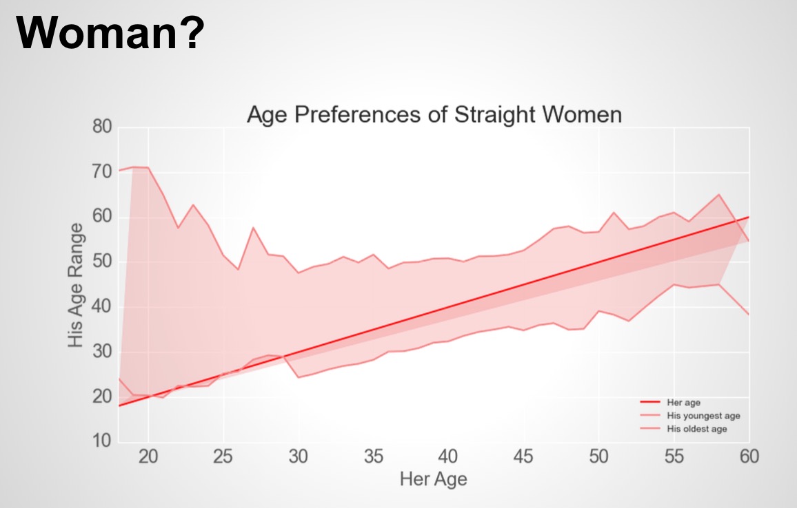
Who do you think is pickier in terms of the age preferences? Men or Women? What are the age preferences users indicated in their profiles compared to their own age? Are they looking for older people or younger people? The following plots shows that men are actually less sensitive to girls’ ages, at least in my dataset. And the group of younger bisexual users know who they are looking for the most specifically.

# straight men age range plot
young = []
old = []
for i in p.index:
   y = int(re.findall('(\d\d)–', p.ages[i])[0])
   o = int(re.findall('–(\d\d)', p.ages[i])[0])
   young.append(y)
   old.append(o)
young = pd.Series(young)
old = pd.Series(old)
agerange = pd.DataFrame(p.age, columns=['age'])
agerange['young'] = young
agerange['old'] = old
print len(agerange)

plt.rcParams['figure.figsize'] = 12, 6
plot = agerange.groupby(agerange.age).mean()
plt.plot(plot.index, plot.index, color='blue', label = 'His age')
plt.plot(plot.index, plot.young, color='dodgerblue', label = 'Her youngest age')
plt.plot(plot.index, plot.old, color='dodgerblue', label = 'Her oldest age')
plot.old[18] = 18
plot.young[99] = 99
plt.fill(plot.index, plot.old, color='dodgerblue', alpha = 0.3)
plt.fill(plot.index, plot.young, color='dodgerblue', alpha = 0.3)
plt.xlabel('His Age', fontsize = 20)
plt.ylabel('Her Age Range', fontsize = 20)
plt.xticks(np.arange(20,85,5), fontsize=20)
plt.yticks(fontsize=20)
plt.title('Age Preferences of Straight Men', fontsize = 25)
plt.xlim(18,60)
plt.legend(loc = 4)

# straight women age range plot
young = []
old = []
for i in p2.index:
   y = int(re.findall('(\d\d)–', p2.ages[i])[0])
   o = int(re.findall('–(\d\d)', p2.ages[i])[0])
   young.append(y)
   old.append(o)
young = pd.Series(young)
old = pd.Series(old)
agerange = pd.DataFrame(p2.age, columns=['age'])
agerange['young'] = young
agerange['old'] = old
print len(agerange)
plot = agerange.groupby(agerange.age).mean()
plot = plot.loc[plot.index <= 60,]

plt.rcParams['figure.figsize'] = 12, 6
plt.plot(plot.index, plot.index, color='red', label = 'Her age')
plt.plot(plot.index, plot.young, color='#F08080', label = 'His youngest age')
plt.plot(plot.index, plot.old, color='#F08080', label = 'His oldest age')
plot.loc[18] = 18
plot.young[60] = 60
plt.fill(plot.index, plot.old, color='#F08080', alpha = 0.3)
plt.fill(plot.index, plot.young, color='#F08080', alpha = 0.3)
plt.xlabel('Her Age', fontsize = 20)
plt.ylabel('His Age Range', fontsize = 20)
plt.xticks(np.arange(20,85,5), fontsize=20)
plt.yticks(fontsize=20)
plt.title('Age Preferences of Straight Women', fontsize = 25)
plt.xlim(18,60)
plt.legend(loc = 4)

# bisexual mixed gender age range plot
young = []
old = []
for i in p3.index:
   y = int(re.findall('(\d\d)–', p3.ages[i])[0])
   o = int(re.findall('–(\d\d)', p3.ages[i])[0])
   young.append(y)
   old.append(o)
young = pd.Series(young)
old = pd.Series(old)
agerange = pd.DataFrame(p3.age, columns=['age'])
agerange['young'] = young
agerange['old'] = old
print len(agerange)
plot = agerange.groupby(agerange.age).mean()
plot = plot.loc[plot.index <= 60,]

plt.rcParams['figure.figsize'] = 12, 6
plt.plot(plot.index, plot.index, color='purple', label = 'His/Her age')
plt.plot(plot.index, plot.young, color='mediumpurple', label = 'His/Her youngest age')
plt.plot(plot.index, plot.old, color='mediumpurple', label = 'His/Her oldest age')
plot.loc[18] = 18
plot.old[57] = 57
plot.young[57] = 57
plt.fill(plot.index, plot.old, color='mediumpurple', alpha = 0.3)
plt.fill(plot.index, plot.young, color='mediumpurple', alpha = 0.3)
plt.xlabel('His/Her Age', fontsize = 20)
plt.ylabel('His/Her Age Range', fontsize = 20)
plt.xticks(np.arange(20,85,5), fontsize=20)
plt.yticks(fontsize=20)
plt.title('Age Preferences of Bisexual Mixed Gender Users', fontsize = 25)
plt.xlim(18,60)
plt.legend(loc = 4)

Who is lying?

Who do you think is taller online than reality? Men or Women? It’s interesting that compared to the data from CDC paper (source), men that are 20 years and older have an average of 5 cm or 2 inches taller heights on their OkCupid profiles. If you look at the blue shape carefully, the first place that is missing is between 5’8” and 5’9”, whereas the peak goes up quickly around 6 feet area. Should we really trust people who claim they are 6 feet tall on OkCupid now??

Well, although there is a chance that people are really lying about their heights (source), I’m not saying that it is definite. The factors contributing to the height differences could also be: 1) Biased data collection. 2) People who use Okcupid really are taller than the average!

%pylab inline
# straight man height plot
man = p[(p.gender == 'Man') & (p.age >= 20)]
lst=[]
count = 0
for i in man.height:
   if type(i) == str:
   lst.append(int(float(re.findall('(\d.\d\d)m', i)[0])*100))
   count += 1
print count
lst = pd.Series(lst)

plt.rcParams['figure.figsize'] = 12, 6
sns.kdeplot(lst, shade=True, label='Self-reported Height on Okcupid (20 years and older)', color = 'dodgerblue')
seq = np.linspace(130,220,100)
plt.plot(seq, stats.norm.pdf(seq, loc =175.9, scale = np.sqrt(5647)*0.2/2), color='red', label = 'Average Height from CDC (20 years and older)')
plt.legend(loc = 1)
plt.xticks(np.arange(140,220,5), fontsize=15)
plt.yticks(fontsize=20)
plt.xlabel('Height(cm)', fontsize = 20)
plt.ylabel('Density', fontsize = 20)
plt.title('Average Height of Men Compared to Reality', fontsize = 25)
plt.xlim(18,60)
plt.legend(loc = 1)
plt.xlim(145, 210)

# straight woman height plot
woman = p2[(p2.gender == 'Woman') & (p2.age >= 20)]
lst=[]
count = 0
for i in woman.height:
   if type(i) == str:
   lst.append(int(float(re.findall('(\d.\d\d)m', i)[0])*100))
   count += 1
print count
lst = pd.Series(lst)

plt.rcParams['figure.figsize'] = 12, 6
sns.kdeplot(lst, shade=True, label='Self-reported Height on Okcupid (20 years and older)', color = '#F08080')
seq = np.linspace(130,220,100)
plt.plot(seq, stats.norm.pdf(seq, loc =162.1, scale = np.sqrt(5971)*0.14/1.5), color='red', label = 'Average Height from CDC (20 years and older)')
plt.legend(loc = 1)
plt.xticks(np.arange(140,220,5), fontsize=15)
plt.yticks(fontsize=20)
plt.xlabel('Height(cm)', fontsize = 20)
plt.ylabel('Density', fontsize = 20)
plt.title('Average Height of Women Compared to Reality', fontsize = 25)
plt.xlim(18,60)
plt.legend(loc = 1)
plt.xlim(140, 210)